Ask-and-tell: How to use Optuna with Spark

Optuna is a hyperparameter optimisation framework that implements a variety of efficient sampling algorithms. Although using Spark to distribute the optimisation task is not part of Optuna’s API, it’s relatively straightforward to do batch optimisation using the ‘ask-and-tell interface’. The Hyperopt Python package does have Spark support but it also requires Hyperopt to be installed on the Spark executors. Moreover, Optuna has some nice features that Hyperopt does not have. In this blogpost I show how to do use Optuna with Spark.

First, we create a spark session and load the California housing dataset from scikit-learn that we will use for demonstation. To speed things up, we take a sample of 1,000 rows from this dataset.

spark = SparkSession.builder.getOrCreate()

from sklearn.datasets import fetch_california_housing

df = pd.concat(fetch_california_housing(as_frame=True, return_X_y=True), axis=1)
df = df.sample(n=1000, random_state=0)

target = 'MedHouseVal'
features = df.drop(columns=[target]).columns.to_list()

We’re going to hyperparameter tune an XGBoost regression model. The hyperparameters that we tune are the learning rate, the maximum tree depth, the number of estimators and the L1 (alpha) en L2 (lambda) regularisation parameters. We create a function that takes a single set of hyperpameter values and that returns the mean of cross validation calculated scores. To calculate these, we use scikit-learn’s cross_validate function. By convention, ‘scores’ in scikit-learn require higher values to be better, so that’s why we need the negative version of the root mean squared error. This function will be run on the executors of the Spark cluster.

from xgboost import XGBRegressor
from sklearn.model_selection import cross_validate


def calculate_objective(learning_rate, max_depth, n_estimators, reg_alpha, reg_lambda):
    estimator = XGBRegressor(learning_rate=learning_rate,
                             max_depth=max_depth,
                             n_estimators=n_estimators,
                             reg_alpha=reg_alpha,
                             reg_lambda=reg_lambda)
    result = cross_validate(estimator, 
                            df[features], 
                            df[target], 
                            scoring='neg_root_mean_squared_error')
    return result['test_score'].mean()

Now we need to define the search space of the hyperparameters and parallelise the calculation. The Tree-structured Parzen Estimator is Optuna’s default sampler. A good exlanation on this algorithm can be found here. The first step in this algorithm is random sampling hyperparameter combinations and calculating the cost function for each. Setting the number of randomly sampled hyperparameters to a large value reduces the probability of ending up in a local optimum instead of the desired global optimum. As I’m running this locally, the ‘cluster’ contains only 8 executors so we set the batch size to 8. Let’s say we want to evaluate 50 batches of which the first 20 are to ‘startup’; these are randomly drawn hyperparameter combinations. As we use the negative mean squared error as cost function, we need to tell Optuna to maximize its value. Optuna documentation advises to set constant_liar to True for batch optimisation. This will avoid multiple executors to evaluate very similar hyperparameter combinations.

We provide all random hyperparameter combinations at once to the Spark cluster and not in batches of 8. This way, we don’t need to wait for the slowest of the 8 evaluations to be finished before continuing with the next set; all executors will be used until all random hyperparameter combinations are evaluated. To get hyperparameter combinations to be evaluated, the Study instance has an ask method. The result should be provided to the Study instance using the tell method. After the startup trials, we ask for new hyperparameter sets after each batch of 8 evaluations in order take advantage of the Optuna’s optimisation algorithm.

def objective_spark(trials):
    params = [[t.suggest_float("learning_rate", 0.01, 0.5),
               t.suggest_int("max_depth", 1, 100),
               t.suggest_int("n_estimators", 2, 1000),
               t.suggest_float("reg_alpha", 0, 10),
               t.suggest_float("reg_lambda", 0, 10),               
              ] for t in trials]
    rdd = spark.sparkContext.parallelize(params, len(params))
    rdd_map_result = rdd.map(lambda p: calculate_objective(*p)).collect()
    return rdd_map_result

n_batches = 50
batch_size = 8
n_startup_batches = 20
n_startup_trials = n_startup_batches*batch_size
study = optuna.create_study(
    sampler=optuna.samplers.TPESampler(n_startup_trials=n_startup_trials,
                                       constant_liar=True),
    direction='maximize')

# First get results for random hyperparameter combinations
startup_trials = [study.ask() for _ in range(n_startup_trials)]
startup_trial_numbers = [t.number for t in startup_trials]
startup_results = objective_spark(startup_trials)

for startup_trial_number, startup_result in zip(startup_trial_numbers, startup_results):
    study.tell(startup_trial_number, startup_result)
print("After random parameter combinations:")
print('Best parameters:', study.best_params, "Best value:", study.best_value)

# Let the Tree-structured Parzen Estimator come up with combinations to try
for j in range(n_startup_batches, n_batches):
    trials = [study.ask() for _ in range(batch_size)]
    trial_numbers = [t.number for t in trials]
    batch_results = objective_spark(trials)
 
    for trial_number, batch_result in zip(trial_numbers, batch_results):
        study.tell(trial_number, batch_result)
    print(j, study.best_params, study.best_value)

[I 2025-05-05 11:13:14,695] A new study created in memory with name: no-name-1d64bda7-4ba9-4d50-b0e1-6d9c264908b7
                                                                                                                                                                                                                                                                                                                                                                                                                                                                                                                                                                                                                                                                                                                                                                                                                                                                                                                                                                                                                                                                                                                                                                                                                                                                                                                                                                                                                                                                                                                                                                                                                                                                                                                                                                                                                                                                                                                                                                                                                                                                                                                                                                                                                                                                                                                                                                                                                                                                                                [Stage 31:====================================>                     (5 + 3) / 8]                                                                                

After random parameter combinations:
Best parameters: {'learning_rate': 0.1311691081810965, 'max_depth': 4, 'n_estimators': 664, 'reg_alpha': 1.6891693775759897, 'reg_lambda': 6.437762039469144} Best value: -0.5793585810589204
20 {'learning_rate': 0.13104804160265776, 'max_depth': 3, 'n_estimators': 531, 'reg_alpha': 2.0165029530049488, 'reg_lambda': 5.766756295911177} -0.5758648464241053
21 {'learning_rate': 0.08633253284746877, 'max_depth': 4, 'n_estimators': 467, 'reg_alpha': 2.1181398204415176, 'reg_lambda': 5.126682207615397} -0.5747320503447746
22 {'learning_rate': 0.08633253284746877, 'max_depth': 4, 'n_estimators': 467, 'reg_alpha': 2.1181398204415176, 'reg_lambda': 5.126682207615397} -0.5747320503447746
23 {'learning_rate': 0.08633253284746877, 'max_depth': 4, 'n_estimators': 467, 'reg_alpha': 2.1181398204415176, 'reg_lambda': 5.126682207615397} -0.5747320503447746
24 {'learning_rate': 0.08633253284746877, 'max_depth': 4, 'n_estimators': 467, 'reg_alpha': 2.1181398204415176, 'reg_lambda': 5.126682207615397} -0.5747320503447746
25 {'learning_rate': 0.08633253284746877, 'max_depth': 4, 'n_estimators': 467, 'reg_alpha': 2.1181398204415176, 'reg_lambda': 5.126682207615397} -0.5747320503447746
26 {'learning_rate': 0.08633253284746877, 'max_depth': 4, 'n_estimators': 467, 'reg_alpha': 2.1181398204415176, 'reg_lambda': 5.126682207615397} -0.5747320503447746
27 {'learning_rate': 0.08633253284746877, 'max_depth': 4, 'n_estimators': 467, 'reg_alpha': 2.1181398204415176, 'reg_lambda': 5.126682207615397} -0.5747320503447746
28 {'learning_rate': 0.07879549009985837, 'max_depth': 4, 'n_estimators': 642, 'reg_alpha': 1.8414509615112093, 'reg_lambda': 5.6157124301959165} -0.5724592058132169
29 {'learning_rate': 0.05979444899483358, 'max_depth': 4, 'n_estimators': 484, 'reg_alpha': 1.6687887588362003, 'reg_lambda': 5.999394259430553} -0.5721387540445764
30 {'learning_rate': 0.05979444899483358, 'max_depth': 4, 'n_estimators': 484, 'reg_alpha': 1.6687887588362003, 'reg_lambda': 5.999394259430553} -0.5721387540445764
31 {'learning_rate': 0.05979444899483358, 'max_depth': 4, 'n_estimators': 484, 'reg_alpha': 1.6687887588362003, 'reg_lambda': 5.999394259430553} -0.5721387540445764
32 {'learning_rate': 0.0476114535610188, 'max_depth': 4, 'n_estimators': 473, 'reg_alpha': 1.580842456659082, 'reg_lambda': 5.086107195414869} -0.570046250869071
33 {'learning_rate': 0.0476114535610188, 'max_depth': 4, 'n_estimators': 473, 'reg_alpha': 1.580842456659082, 'reg_lambda': 5.086107195414869} -0.570046250869071
34 {'learning_rate': 0.0476114535610188, 'max_depth': 4, 'n_estimators': 473, 'reg_alpha': 1.580842456659082, 'reg_lambda': 5.086107195414869} -0.570046250869071
35 {'learning_rate': 0.0476114535610188, 'max_depth': 4, 'n_estimators': 473, 'reg_alpha': 1.580842456659082, 'reg_lambda': 5.086107195414869} -0.570046250869071
36 {'learning_rate': 0.0476114535610188, 'max_depth': 4, 'n_estimators': 473, 'reg_alpha': 1.580842456659082, 'reg_lambda': 5.086107195414869} -0.570046250869071
37 {'learning_rate': 0.0476114535610188, 'max_depth': 4, 'n_estimators': 473, 'reg_alpha': 1.580842456659082, 'reg_lambda': 5.086107195414869} -0.570046250869071
38 {'learning_rate': 0.0476114535610188, 'max_depth': 4, 'n_estimators': 473, 'reg_alpha': 1.580842456659082, 'reg_lambda': 5.086107195414869} -0.570046250869071
39 {'learning_rate': 0.0476114535610188, 'max_depth': 4, 'n_estimators': 473, 'reg_alpha': 1.580842456659082, 'reg_lambda': 5.086107195414869} -0.570046250869071
40 {'learning_rate': 0.0476114535610188, 'max_depth': 4, 'n_estimators': 473, 'reg_alpha': 1.580842456659082, 'reg_lambda': 5.086107195414869} -0.570046250869071
41 {'learning_rate': 0.0476114535610188, 'max_depth': 4, 'n_estimators': 473, 'reg_alpha': 1.580842456659082, 'reg_lambda': 5.086107195414869} -0.570046250869071
42 {'learning_rate': 0.0476114535610188, 'max_depth': 4, 'n_estimators': 473, 'reg_alpha': 1.580842456659082, 'reg_lambda': 5.086107195414869} -0.570046250869071
43 {'learning_rate': 0.0476114535610188, 'max_depth': 4, 'n_estimators': 473, 'reg_alpha': 1.580842456659082, 'reg_lambda': 5.086107195414869} -0.570046250869071
44 {'learning_rate': 0.0476114535610188, 'max_depth': 4, 'n_estimators': 473, 'reg_alpha': 1.580842456659082, 'reg_lambda': 5.086107195414869} -0.570046250869071
45 {'learning_rate': 0.0476114535610188, 'max_depth': 4, 'n_estimators': 473, 'reg_alpha': 1.580842456659082, 'reg_lambda': 5.086107195414869} -0.570046250869071
46 {'learning_rate': 0.0476114535610188, 'max_depth': 4, 'n_estimators': 473, 'reg_alpha': 1.580842456659082, 'reg_lambda': 5.086107195414869} -0.570046250869071
47 {'learning_rate': 0.0476114535610188, 'max_depth': 4, 'n_estimators': 473, 'reg_alpha': 1.580842456659082, 'reg_lambda': 5.086107195414869} -0.570046250869071
48 {'learning_rate': 0.0476114535610188, 'max_depth': 4, 'n_estimators': 473, 'reg_alpha': 1.580842456659082, 'reg_lambda': 5.086107195414869} -0.570046250869071
49 {'learning_rate': 0.0476114535610188, 'max_depth': 4, 'n_estimators': 473, 'reg_alpha': 1.580842456659082, 'reg_lambda': 5.086107195414869} -0.570046250869071

Let’s now collect all results in a Pandas dataframe and investigate the results in a parallel coordinates plot.

result_df = pd.DataFrame([x.params for x in study.get_trials()])
result_df['test_score'] = [x.values[0] for x in study.get_trials()]
result_df['iteration'] = [x.number for x in study.get_trials()]
result_df = result_df.sort_values('test_score', ascending=False)

learning_rate	max_depth	n_estimators	reg_alpha	reg_lambda	test_score	iteration
0.047611	4	473	1.580842	5.086107	-0.570046	259
0.055013	4	453	1.637850	4.717187	-0.571130	353
0.054364	4	395	1.201306	4.987839	-0.572038	333
0.059794	4	484	1.668789	5.999394	-0.572139	232
0.040800	4	461	1.912329	5.103767	-0.572192	290

import plotly.express as px

px.parallel_coordinates(result_df[['test_score', 'learning_rate',
                                   'n_estimators', 'max_depth',
                                   'reg_alpha', 'reg_lambda']],
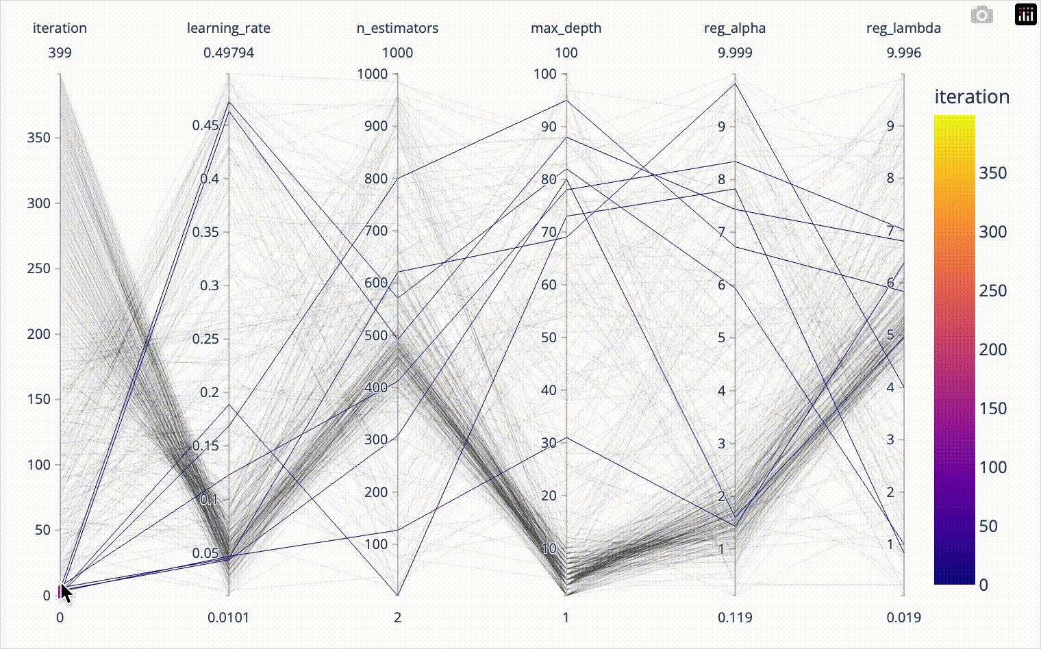
                        color='test_score')

When we include the iteration number in the parallel coordinates plot, we can confirm that the first 20*8=160 iterations were totally random and nicely covered the whole parameter space. Afterwards we see how the algorithm converges towards the optimal hyperparameter combination. The plotly parallel coordinates plot allows for highlighting a subset of values by selecting ranges on the individual axes. I show this in the animation below.

px.parallel_coordinates(result_df[['iteration', 'learning_rate',
                                   'n_estimators', 'max_depth',
                                   'reg_alpha', 'reg_lambda']],
                        color='iteration')